5.4. Other Power Spectral Density estimates
Contents
5.4.1. Covariance method
-
arcovar(x, order)[source]¶ Simple and fast implementation of the covariance AR estimate
This code is 10 times faster than
arcovar_marple()and more importantly only 10 lines of code, compared to a 200 loc forarcovar_marple()Parameters: - X (array) – Array of complex data samples
- oder (int) – Order of linear prediction model
Returns: - a - Array of complex forward linear prediction coefficients
- e - error
The covariance method fits a Pth order autoregressive (AR) model to the input signal, which is assumed to be the output of an AR system driven by white noise. This method minimizes the forward prediction error in the least-squares sense. The output vector contains the normalized estimate of the AR system parameters
The white noise input variance estimate is also returned.
If is the power spectral density of y(n), then:
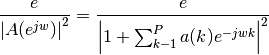
Because the method characterizes the input data using an all-pole model, the correct choice of the model order p is important.
from spectrum import arcovar, marple_data, arma2psd
from pylab import plot, log10, linspace, axis

ar_values, error = arcovar(marple_data, 15)
psd = arma2psd(ar_values, sides='centerdc')
plot(linspace(-0.5, 0.5, len(psd)), 10*log10(psd/max(psd)))
axis([-0.5, 0.5, -60, 0])
(Source code, png, hires.png, pdf)

See also
Validation: the AR parameters are the same as those returned by a completely different function arcovar_marple().References: [Mathworks]
-
arcovar_marple(x, order)[source]¶ Estimate AR model parameters using covariance method
This implementation is based on [Marple]. This code is far more complicated and slower than
arcovar()function, which is now the official version. Seearcovar()for a detailed description of Covariance method.This function should be used in place of arcovar only if order<=4, for which
arcovar()does not work.Fast algorithm for the solution of the covariance least squares normal equations from Marple.
Parameters: - X (array) – Array of complex data samples
- oder (int) – Order of linear prediction model
Returns: - AF - Array of complex forward linear prediction coefficients
- PF - Real forward linear prediction variance at order IP
- AB - Array of complex backward linear prediction coefficients
- PB - Real backward linear prediction variance at order IP
- PV - store linear prediction coefficients
Note
this code and the original code in Marple diverge for ip>10. it seems that this is related to single precision used with complex type in fortran whereas numpy uses double precision for complex type.
Validation: the AR parameters are the same as those returned by a completely different function arcovar().References: [Marple]
-
class
pcovar(data, order, NFFT=None, sampling=1.0, scale_by_freq=False)[source]¶ Class to create PSD based on covariance algorithm
See
arcovar()for description.from spectrum import pcovar, marple_data p = pcovar(marple_data, 15, NFFT=4096) p.plot(sides='centerdc')
(Source code, png, hires.png, pdf)

See also
Constructor
For a detailled description of the parameters, see
arcovar().Parameters:
-
arcovar_marple(x, order)[source] Estimate AR model parameters using covariance method
This implementation is based on [Marple]. This code is far more complicated and slower than
arcovar()function, which is now the official version. Seearcovar()for a detailed description of Covariance method.This function should be used in place of arcovar only if order<=4, for which
arcovar()does not work.Fast algorithm for the solution of the covariance least squares normal equations from Marple.
Parameters: - X (array) – Array of complex data samples
- oder (int) – Order of linear prediction model
Returns: - AF - Array of complex forward linear prediction coefficients
- PF - Real forward linear prediction variance at order IP
- AB - Array of complex backward linear prediction coefficients
- PB - Real backward linear prediction variance at order IP
- PV - store linear prediction coefficients
Note
this code and the original code in Marple diverge for ip>10. it seems that this is related to single precision used with complex type in fortran whereas numpy uses double precision for complex type.
Validation: the AR parameters are the same as those returned by a completely different function arcovar().References: [Marple]
5.4.2. Eigen-analysis methods
-
eigen(X, P, NSIG=None, method='music', threshold=None, NFFT=4096, criteria='aic', verbose=False)[source]¶ Pseudo spectrum using eigenvector method (EV or Music)
This function computes either the Music or EigenValue (EV) noise subspace frequency estimator.
First, an autocorrelation matrix of order P is computed from the data. Second, this matrix is separated into vector subspaces, one a signal subspace and the other a noise subspace using a SVD method to obtain the eigen values and vectors. From the eigen values
 , and eigen vectors
  ,
the pseudo spectrum (see note below) is computed as follows:
,
the pseudo spectrum (see note below) is computed as follows: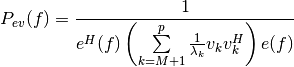
The separation of the noise and signal subspaces requires expertise of the signal. However, AIC and MDL criteria may be used to automatically perform this task.
You still need to provide the parameter P to indicate the maximum number of eigen values to be computed. The criteria will just select a subset to estimate the pseudo spectrum (see
aic_eigen()andmdl_eigen()for details.Note
pseudo spectrum. func:eigen does not compute a PSD estimate. Indeed, the method does not preserve the measured process power.
Parameters: - X – Array data samples
- P (int) – maximum number of eigen values to compute. NSIG (if specified) must therefore be less than P.
- method (str) – ‘music’ or ‘ev’.
- NSIG (int) – If specified, the signal sub space uses NSIG eigen values.
- threshold (float) – If specified, the signal sub space is made of the
eigen values larger than
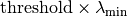 ,
where
,
where  is the minimum eigen values.
 - NFFT (int) – total length of the final data sets (padded with zero if needed; default is 4096)
Returns: - PSD: Array of real frequency estimator values (two sided for
- complex data and one sided for real data)
- S, the eigen values
from spectrum import eigen, marple_data
from pylab import plot, log10, linspace, legend, axis

psd, ev = eigen(marple_data, 15, NSIG=11)
f = linspace(-0.5, 0.5, len(psd))
plot(f, 10 * log10(psd/max(psd)), label='User defined')

psd, ev = eigen(marple_data, 15, threshold=2)
plot(f, 10 * log10(psd/max(psd)), label='threshold method (100)')

psd, ev = eigen(marple_data, 15)
plot(f, 10 * log10(psd/max(psd)), label='AIC method (8)')

legend()
axis([-0.5, 0.5, -120, 0])
(Source code, png, hires.png, pdf)

See also
References: [Marple], Chap 13 Todo
for developers:
- what should be the second argument of the criteria N, N-P, P…?
- what should be the max value of NP
-
class
pev(data, IP, NSIG=None, NFFT=None, sampling=1.0, scale_by_freq=False, threshold=None, criteria='aic', verbose=False)[source]¶ Class to create PSD using ARMA estimator.
See
eigenfre()for description.from spectrum import pev, marple_data p = pev(marple_data, 15, NFFT=4096) p.plot()
(Source code, png, hires.png, pdf)

Constructor:
For a detailed description of the parameters, see
arma_estimate().Parameters: - data (array) – input data (list or numpy.array)
- P (int) – maximum number of eigen values to compute. NSIG (if specified) must therefore be less than P.
- NSIG (int) – If specified, the signal sub space uses NSIG eigen values.
- NFFT (int) – total length of the final data sets (padded with zero if needed; default is 4096)
- sampling (float) – sampling frequency of the input
data.
-
class
pmusic(data, IP, NSIG=None, NFFT=None, sampling=1.0, threshold=None, criteria='aic', verbose=False, scale_by_freq=False)[source]¶ Class to create PSD using ARMA estimator.
See
pmusic()andeigenfre()for description.from spectrum import pmusic, marple_data p = pmusic(marple_data, 15, NFFT=4096) p.plot()
(Source code, png, hires.png, pdf)

Another example using a two sinusoidal components:
n = arange(200)
x = cos(0.257*pi*n) + sin(0.2*pi*n) + 0.01*randn(size(n));
p = pmusic(x, 6,4)
p.plot()
Constructor:
For a detailed description of the parameters, see
arma_estimate().Parameters: - data (array) – input data (list or numpy.array)
- P (int) – maximum number of eigen values to compute. NSIG (if specified) must therefore be less than P.
- NSIG (int) – If specified, the signal sub space uses NSIG eigen values.
- NFFT (int) – total length of the final data sets (padded with zero if needed; default is 4096)
- sampling (float) – sampling frequency of the input
data.
5.4.3. Minimum Variance estimator
Minimum Variance Spectral Estimators
pminvar(data, order[, NFFT, sampling, …]) |
Class to create PSD based on the Minimum variance spectral estimation |
Code author: Thomas Cokelaer, 2011
-
minvar(X, order, sampling=1.0, NFFT=4096)[source]¶ Minimum Variance Spectral Estimation (MV)
This function computes the minimum variance spectral estimate using the Musicus procedure. The Burg algorithm from
arburg()is used for the estimation of the autoregressive parameters. The MV spectral estimator is given by: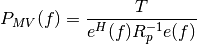
where
 is the inverse of the estimated autocorrelation
matrix (Toeplitz) and
is the inverse of the estimated autocorrelation
matrix (Toeplitz) and  is the complex sinusoid vector.
Parameters: Returns: - PSD - Power spectral density values (two-sided)
- AR - AR coefficients (Burg algorithm)
- k - Reflection coefficients (Burg algorithm)
Note
The MV spectral estimator is not a true PSD function because the area under the MV estimate does not represent the total power in the measured process. MV minimises the variance of the output of a narrowband filter and adpats itself to the spectral content of the input data at each frequency.
Example: The following example computes a PSD estimate using minvar()The output PSD is transformed to acenterdcPSD and plotted.from spectrum import * from pylab import plot, log10, linspace, xlim psd, A, k = minvar(marple_data, 15) psd = twosided_2_centerdc(psd) # switch positive and negative freq f = linspace(-0.5, 0.5, len(psd)) plot(f, 10 * log10(psd/max(psd))) xlim(-0.5, 0.5 )
(Source code, png, hires.png, pdf)

See also
Reference: [Marple]
-
class
pminvar(data, order, NFFT=None, sampling=1.0, scale_by_freq=False)[source]¶ Class to create PSD based on the Minimum variance spectral estimation
See
minvar()for description.from spectrum import * p = pminvar(marple_data, 15, NFFT=4096) p.plot(sides='centerdc')
(Source code, png, hires.png, pdf)

Constructor
For a detailled description of the parameters, see
minvar().Parameters:
5.4.4. Modified Covariance method
Module related to the modcovar methods
-
modcovar(x, order)[source]¶ Simple and fast implementation of the covariance AR estimate
This code is 10 times faster than
modcovar_marple()and more importantly only 10 lines of code, compared to a 200 loc formodcovar_marple()Parameters: - X – Array of complex data samples
- order (int) – Order of linear prediction model
Returns: - P - Real linear prediction variance at order IP
- A - Array of complex linear prediction coefficients
from spectrum import modcovar, marple_data, arma2psd, cshift
from pylab import log10, linspace, axis, plot

a, p = modcovar(marple_data, 15)
PSD = arma2psd(a)
PSD = cshift(PSD, len(PSD)/2) # switch positive and negative freq
plot(linspace(-0.5, 0.5, 4096), 10*log10(PSD/max(PSD)))
axis([-0.5,0.5,-60,0])
(Source code, png, hires.png, pdf)

See also
Validation: the AR parameters are the same as those returned by a completely different function modcovar_marple().References: Mathworks
-
modcovar_marple(X, IP)[source]¶ Fast algorithm for the solution of the modified covariance least squares normal equations.
This implementation is based on [Marple]. This code is far more complicated and slower than
modcovar()function, which is now the official version. Seemodcovar()for a detailed description of Modified Covariance method.Parameters: - X –
- Array of complex data samples X(1) through X(N)
- IP (int) –
- Order of linear prediction model (integer)
Returns: - P - Real linear prediction variance at order IP
- A - Array of complex linear prediction coefficients
- ISTAT - Integer status indicator at time of exit
- for normal exit (no numerical ill-conditioning)
- if P is not a positive value
- if DELTA’ and GAMMA’ do not lie in the range 0 to 1
- if P’ is not a positive value
- if DELTA and GAMMA do not lie in the range 0 to 1
Validation: the AR parameters are the same as those returned by a completely different function
modcovar().Note
validation. results similar to test example in Marple but starts to differ for ip~8. with ratio of 0.975 for ip=15 probably due to precision.
References: [Marple] - X –
-
class
pmodcovar(data, order, NFFT=None, sampling=1.0, scale_by_freq=False)[source]¶ Class to create PSD based on modified covariance algorithm
See
modcovar()for description.Examples
from spectrum import pmodcovar, marple_data
p = pmodcovar(marple_data, 15, NFFT=4096)
p.plot(sides='centerdc')
(Source code, png, hires.png, pdf)

See also
Constructor
For a detailled description of the parameters, see
modcovar().Parameters: